Forecasting inflation with AutoML in Amazon SageMaker Autopilot

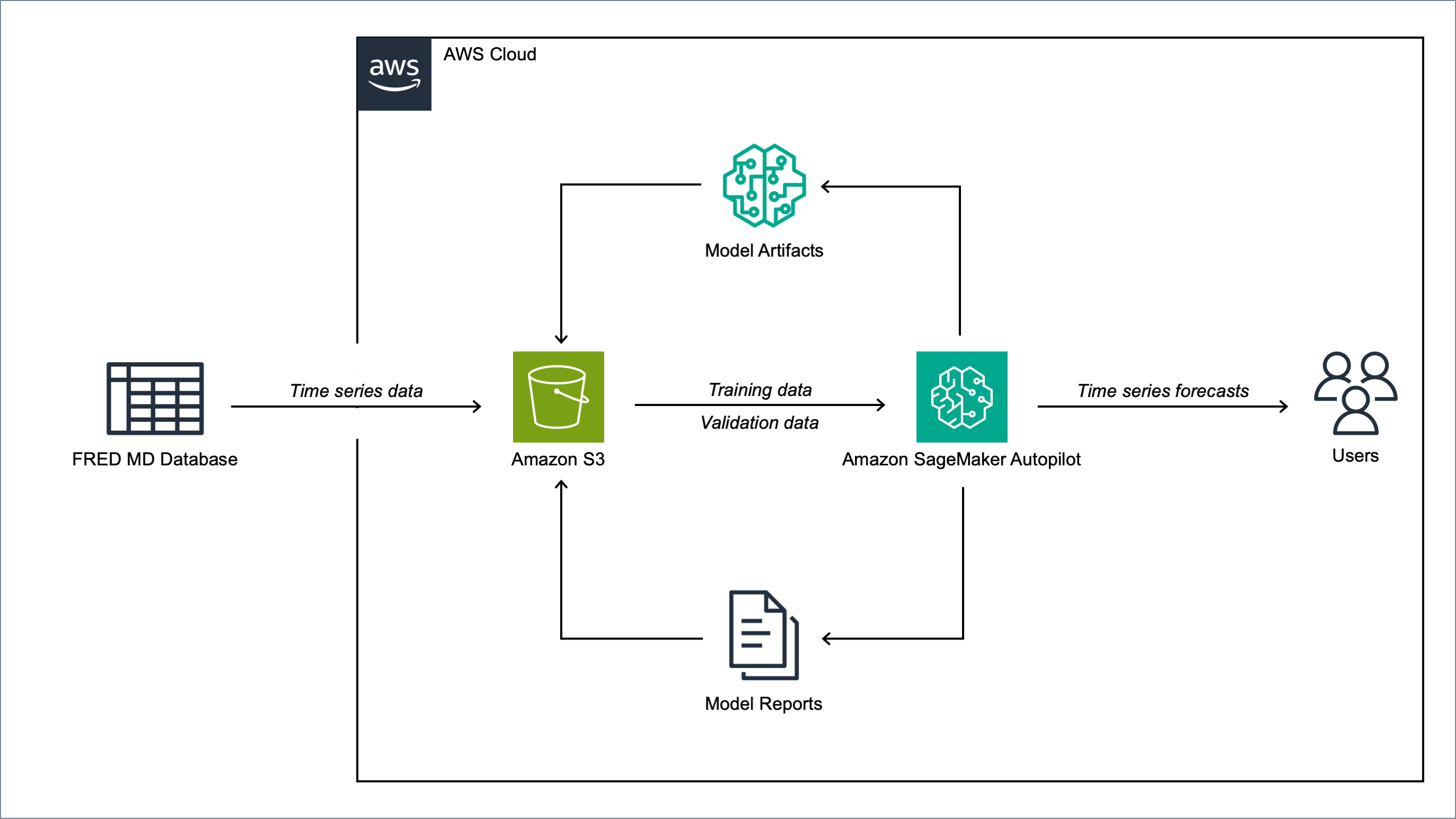
1. Overview

Automated Machine Learning (AutoML) frameworks address the expertise- and time-intensive nature of the traditional ML model development workflow. By automating the end-to-end process of building, training and tuning ML models through easy-to-use programmatic interfaces, AutoML solutions make ML accessible to non-specialists and significantly reduce deployment timeframes.

In this post, we demonstrate how to use Amazon SageMaker Autopilot [1], AWS’s AutoML framework, to forecast US inflation using the FRED-MD dataset [2]. FRED-MD is an open-source dataset maintained by the Federal Reserve Bank of St. Louis including over 100 monthly time series of US macroeconomic indicators (see the Appendix for the full list). FRED-MD is widely used in economic research, and has become a standard benchmark for evaluating machine learning models for US inflation forecasting (see, for instance, [3], [4], [5]).

In this demonstration, we use AutoML to forecast the month-on-month (MoM) US CPI inflation. On each month, the model predicts the following month’s percentage change in the US Consumer Price Index (CPI) using the current month’s FRED-MD indicators as inputs. We first run an AutoML job on FRED-MD data from January 1960 to December 2023 to select the best ML pipeline. We then use this ML pipeline in an Amazon SageMaker batch transform job to generate one-month-ahead forecasts from January 2024 to December 2024.

1.1 Amazon SageMaker Autopilot

Autopilot is a fully managed AutoML solution designed to automate the end-to-end ML pipeline while maintaining transparency and flexibility. Unlike traditional black-box AutoML systems, Autopilot provides a white-box approach, allowing users to inspect and modify the generated ML pipelines to incorporate domain expertise when necessary [1].

Given a tabular dataset and a specified target column, Autopilot generates a set of candidate ML pipelines optimized for the given dataset’s characteristics and the specific problem type. Each candidate pipeline implements the end-to-end process of data preparation, feature selection and algorithm training. Autopilot then evaluates the candidate pipelines to produce a leaderboard and select the best-performing pipeline.

As part of this process, Autopilot automatically generates a set of data analysis and model insights reports in various formats, along with Jupyter notebooks that allow users to examine and refine the pipelines without reverting to a fully manual approach. Autopilot’s full integration with the broader SageMaker platform allows users to quickly deploy the final selected pipeline in production.

1.2 FRED-MD dataset

FRED-MD is a publicly available dataset of U.S. macroeconomic indicators maintained by the Federal Reserve Bank of St. Louis. The FRED-MD dataset was introduced to provide a common benchmark for comparing model performance and to facilitate the reproducibility of research results [2].

The FRED-MD dataset is updated on a monthly basis, with each monthly release referred to as vintage. The vintages are published on the FRED-MD website in CSV format. Each vintage includes monthly data from January 1959 up to the month prior to the release. For instance, the January 2024 vintage includes the data from January 1959 to December 2023. Different vintages can include different time series, as indicators are occasionally added and removed from the dataset.

The FRED-MD time series are sourced from the Federal Reserve Economic Data (FRED) database, which is St. Louis Fed’s main, publicly accessible, economic database. Different retrospective adjustments are applied to the time series sourced from the FRED database, including seasonal adjustments, inflation adjustments and backfilling of missing values. As a result, different vintages can report different values for the same time series on the same date.

The FRED-MD dataset has been used extensively for forecasting US inflation. In [3] it was shown that a random forest model trained on the FRED-MD dataset outperforms several standard inflation forecasting models at different forecasting horizons. [4] applied different dimension reduction techniques to the FRED-MD dataset to forecast US inflation and found that autoencoders provide the best performance. [5] expanded the analysis in [3] to include an LSTM model and found that it did not significantly outperform the random forest model.

2. Solution

Note

To be able to run the code provided in this section, you will need to launch an Amazon SageMaker notebook instance. You will also need to download the CSV files with the FRED-MD data from the FRED-MD website and store them in a local folder.

2.1 Set up the environment

We start by importing all the dependencies and setting up the Amazon SageMaker environment.

# Import the dependencies
import io
import json
import sagemaker
import pandas as pd
import numpy as np
import matplotlib.pyplot as plt
from sklearn.metrics import root_mean_squared_error, mean_absolute_error

# Get the SageMaker session
session = sagemaker.Session()

# Get the SageMaker execution role
role = sagemaker.get_execution_role()

# Get the default S3 bucket
bucket = session.default_bucket()

2.2 Define the auxiliary functions for working with the FRED-MD data

Next, we define a set of auxiliary functions for processing the FRED-MD data.

2.2.1 transform_series

The transform_series function transforms each FRED-MD time series according to the assigned transformation code. The transformation code specifies which transformation the FRED-MD authors suggest applying to each time series in order to make it stationary. The transformation codes are included in the first row of each CSV file and are defined as follows:

1. no transformation

2. first order difference

3. second order difference

4. logarithm

5. first order logarithmic difference

6. second order logarithmic difference

7. percentage change

def transform_series(
    x,
    tcode
):
    """
    Transform the time series.

    Parameters:
    ========================================================================================================
    x: pandas.Series
        Time series.

    tcode: int.
        Transformation code.
    """

    if tcode == 1:
        # No transformation
        return x

    elif tcode == 2:
        # First order absolute difference
        return x.diff()

    elif tcode == 3:
        # Second order absolute difference
        return x.diff().diff()

    elif tcode == 4:
        # Logarithm
        return np.log(x)

    elif tcode == 5:
        # First order logarithmic difference
        return np.log(x).diff()

    elif tcode == 6:
        # Second order logarithmic difference
        return np.log(x).diff().diff()

    elif tcode == 7:
        # Percentage change
        return x.pct_change()

    else:
        raise ValueError(f"unknown `tcode` {tcode}")

2.2.2 get_data

The get_data function loads the data for a selected vintage from the corresponding CSV file and prepares it for the model by transforming and lagging the time series.

def get_data(
    vintage,
    series_names,
    target_name,
    target_tcode,
    n_lags,
):
    """
    Get the data for a selected vintage.

    Parameters:
    ========================================================================================================
    vintage: str.
        The vintage of the dataset, in "YYYY-MM" format.

    series_names: str.
        The time series to be included in the dataset.

    target_name: string.
        The name of the target time series.

    target_tcode: int.
        The transformation code of the target time series.

    n_lags: int.
        The number of autoregressive lags.
    """
    # Get the file path
    file = f"data/{vintage}.csv"

    # Get the time series
    data = pd.read_csv(file, skiprows=list(range(1, 11)), index_col=0)
    data.index = pd.to_datetime(data.index)
    data.columns = [c.upper() for c in data.columns]
    data = data.loc[:, series_names]

    # Get the transformation codes
    tcodes = pd.read_csv(file, nrows=1, index_col=0)
    tcodes.columns = [c.upper() for c in tcodes.columns]

    # Override the target's transformation code
    tcodes[target_name] = target_tcode

    # Transform the time series
    data = data.apply(lambda x: transform_series(x, tcodes[x.name].item()))

    # Add the lags
    data = data[[target_name]].join(data.shift(periods=list(range(1, 1 + n_lags)), suffix="_LAG"))

    # Drop the missing values resulting from applying the transformations and taking the lags
    data = data.dropna()

    return data

2.2.3 get_common_series

To ensure consistent data across training, validation, and testing, we define a function that identifies which indicators have complete time series across all consecutive vintages in our analysis period.

def get_common_series(
    start_vintage,
    end_vintage
):
    """
    Get the list of complete time series included in all dataset releases between two vintages.

    Parameters:
    ========================================================================================================
    start_vintage: str.
        The first vintage, in "YYYY-MM" format.

    end_vintage: str.
        The last vintage, in "YYYY-MM" format.
    """
    # Generate the date range
    dates = pd.date_range(
        start=f"{start_vintage.split('-')[0]}-{start_vintage.split('-')[1]}-01",
        end=f"{end_vintage.split('-')[0]}-{end_vintage.split('-')[1]}-01",
        freq="MS"
    )

    # Create a list for storing the names of the complete time series
    series = []

    # Loop across the dates
    for date in dates:
        # Load the data for the considered date
        data = pd.read_csv(f"data/{date.year}-{format(date.month, '02d')}.csv", skiprows=list(range(1, 11)), index_col=0)

        # Drop the incomplete time series
        data = data.loc[:, data.isna().sum() == 0]

        # Save the names of the complete time series
        series.append([c.upper() for c in data.columns])

    # Get the list of complete time series included in the dataset on all dates
    series = list(set.intersection(*map(set, series)))

    return series

2.2.4 get_real_time_data

To address any potential data leakage, while replicating realistic model usage where the model makes predictions on newly available data, we construct our evaluation set using the last month from each consecutive vintage.

This approach is implemented in the get_real_time_data function, which processes each vintage using the get_data function and concatenates the final month from each vintage into a unique Pandas DataFrame.

def get_real_time_data(
    start_vintage,
    end_vintage,
    series_names,
    target_name,
    target_tcode,
    n_lags,
):

    """
    Get the real-time data between two vintages.

    Parameters:
    ========================================================================================================
    start_vintage: str.
        The first vintage, in "YYYY-MM" format.

    end_vintage: str.
        The last vintage, in "YYYY-MM" format.

    series_names: str.
        The time series to be included in the dataset.

    target_name: string.
        The name of the target time series.

    target_tcode: int.
        The transformation code of the target time series.

    n_lags: int.
        The number of autoregressive lags.
    """

    # Generate the date range
    dates = pd.date_range(
        start=f"{start_vintage.split('-')[0]}-{start_vintage.split('-')[1]}-01",
        end=f"{end_vintage.split('-')[0]}-{end_vintage.split('-')[1]}-01",
        freq="MS"
    )

    # Get the last month of data for each date in the considered range
    data = pd.concat([
        get_data(
            vintage=f"{date.year}-{format(date.month, '02d')}",
            series_names=series_names,
            target_name=target_name,
            target_tcode=target_tcode,
            n_lags=n_lags,
        ).iloc[-1:]
        for date in dates
    ])

    return data

2.3 Prepare the FRED-MD data and upload it to S3

We now use the functions defined in the previous section for processing the FRED-MD data. We start by defining the target name, the target transformation code and the number of lags used for constructing the features.

Note

We override the suggested transformation for the US CPI, which is second order logarithmic difference (tcode = 6), as the resulting time series can’t be interpreted as an inflation rate. We use percentage changes (tcode = 7) instead, which results in a MoM inflation rate time series.

# Define the name of the target time series
target_name = "CPIAUCSL"

# Define the transformation code of the target time series
target_tcode = 7

# Define the number of autoregressive lags of each time series
n_lags = 1

After that, we extract the list of complete time series included in all vintages used for the analysis.

# Get the list of complete time series included in all vintages from 2023-01 to 2025-01
series_names = get_common_series(
    start_vintage="2023-01",
    end_vintage="2025-01",
)

This results in 101 time series, including the target time series.

2.3.1 Training data

For training the candidate models during the AutoML experiment, we use the data from January 1960 to December 2022.

# Prepare the training data
training_data = get_data(
    vintage="2023-01",
    series_names=series_names,
    target_name=target_name,
    target_tcode=target_tcode,
    n_lags=n_lags,
)

# Upload the training data to S3
training_data_s3_uri = session.upload_string_as_file_body(
    body=training_data.to_csv(index=False),
    bucket=bucket,
    key="data/train.csv"
)

2.3.2 Validation data

For evaluating and ranking the candidate models during the AutoML experiment, we use the data from January 2023 to December 2023, where the data for each month is extracted separately from the corresponding vintage.

Important

If the validation data is not provided, SageMaker Autopilot performs cross-validation on the training data. However, the generated cross-validation splits may not preserve temporal order, resulting in potentially training the model on future data and evaluating it on past data.

# Prepare the validation data
validation_data = get_real_time_data(
    start_vintage="2023-02",
    end_vintage="2024-01",
    series_names=series_names,
    target_name=target_name,
    target_tcode=target_tcode,
    n_lags=n_lags,
)

# Upload the validation data to S3
validation_data_s3_uri = session.upload_string_as_file_body(
    body=validation_data.to_csv(index=False),
    bucket=bucket,
    key="data/valid.csv"
)

2.3.3 Test data

For testing the best candidate model selected by the AutoML experiment, we use the data from January 2024 to December 2024, where again the data for each month is extracted separately from the corresponding vintage. The testing is performed later by performing a batch transform job with the best candidate model to generate the test set predictions.

Important

Make sure to exclude the header and to drop the target column from the test dataset before uploading it to S3, otherwise the batch transform job will fail.

# Prepare the test data
test_data = get_real_time_data(
    start_vintage="2024-02",
    end_vintage="2025-01",
    series_names=series_names,
    target_name=target_name,
    target_tcode=target_tcode,
    n_lags=n_lags,
)

# Upload the test data to S3
test_data_s3_uri = session.upload_string_as_file_body(
    body=test_data.drop(labels=[target_name], axis=1).to_csv(index=False, header=False),
    bucket=bucket,
    key="data/test.csv"
)

2.4 Configure and run the AutoML job

We configure the AutoML experiment as a regression task, using mean squared error (MSE) as the validation objective to minimize. The experiment is run in ensembling mode, so the final pipeline combines multiple algorithms rather than returning a single optimized model.

# Define the AutoML job configuration
automl = sagemaker.automl.automlv2.AutoMLV2(
    problem_config=sagemaker.automl.automlv2.AutoMLTabularConfig(
        target_attribute_name=target_name,
        algorithms_config=["randomforest", "extra-trees", "xgboost", "linear-learner", "nn-torch"],
        mode="ENSEMBLING",
        problem_type="Regression",
    ),
    job_objective={"MetricName": "MSE"},
    base_job_name="us-cpi",
    output_path=f"s3://{bucket}/output/",
    role=role,
    sagemaker_session=session,
)

# Run the AutoML job
automl.fit(
    inputs=[
        sagemaker.automl.automlv2.AutoMLDataChannel(
            s3_data_type="S3Prefix",
            s3_uri=training_data_s3_uri,
            channel_type="training",
            compression_type=None,
            content_type="text/csv;header=present"
        ),
        sagemaker.automl.automlv2.AutoMLDataChannel(
            s3_data_type="S3Prefix",
            s3_uri=validation_data_s3_uri,
            channel_type="validation",
            compression_type=None,
            content_type="text/csv;header=present"
        ),
    ]
)

After the AutoML job has completed, we can extract the S3 location containing the model artifacts of the final selected pipeline.

# Get the best model
automl.best_candidate()

The AutoML job automatically generates several reports for each candidate pipeline, including a model explainability report with the feature importances and a model quality report with an analysis of the performance on the validation data, which are also saved to S3.

2.4.1 Model explainability report

The model explainability report includes the feature importances calculated using the Kernel SHAP method. The report shows that the previous month’s CPI inflation is the most influential predictor, followed by the industrial production for residential utilities and the crude oil price. Transportation inflation and producer prices for finished consumer goods are also important, while factors such as initial unemployment claims, the AAA corporate bond spread, and real money supply are also relevant, though less significant.

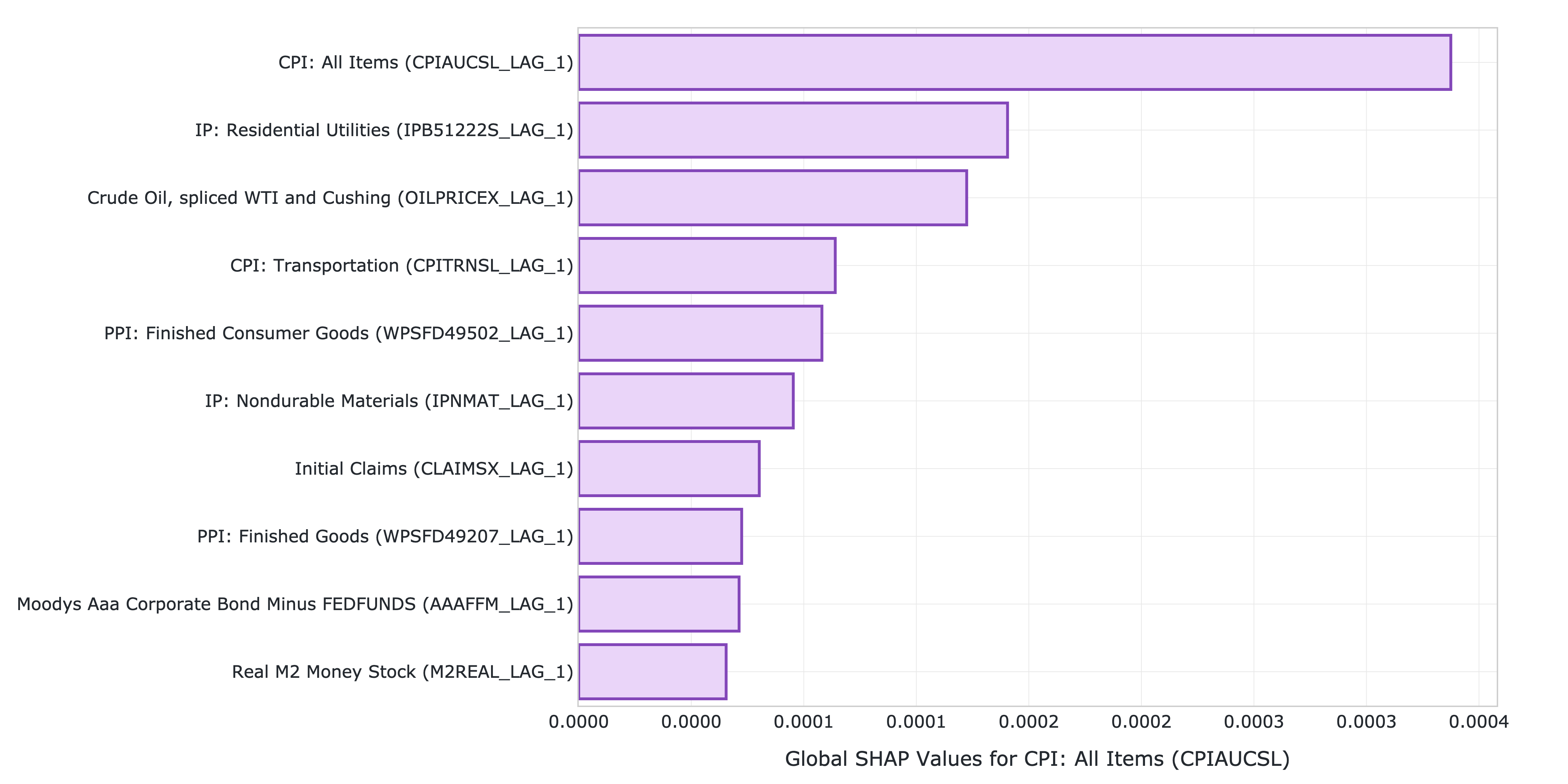
Figure 1: Top 10 features by SHAP value.

2.4.2 Model quality report

The model quality report includes the model’s performance metrics on the validation data as well as several diagnostic plots, such as actual versus predicted scatter plots and standardized residuals plots. The report shows that the model achieves a root mean squared error (RMSE) of 0.2073%, a mean absolute error (MAE) of 0.1743% and a 60% R-squared on the validation data.

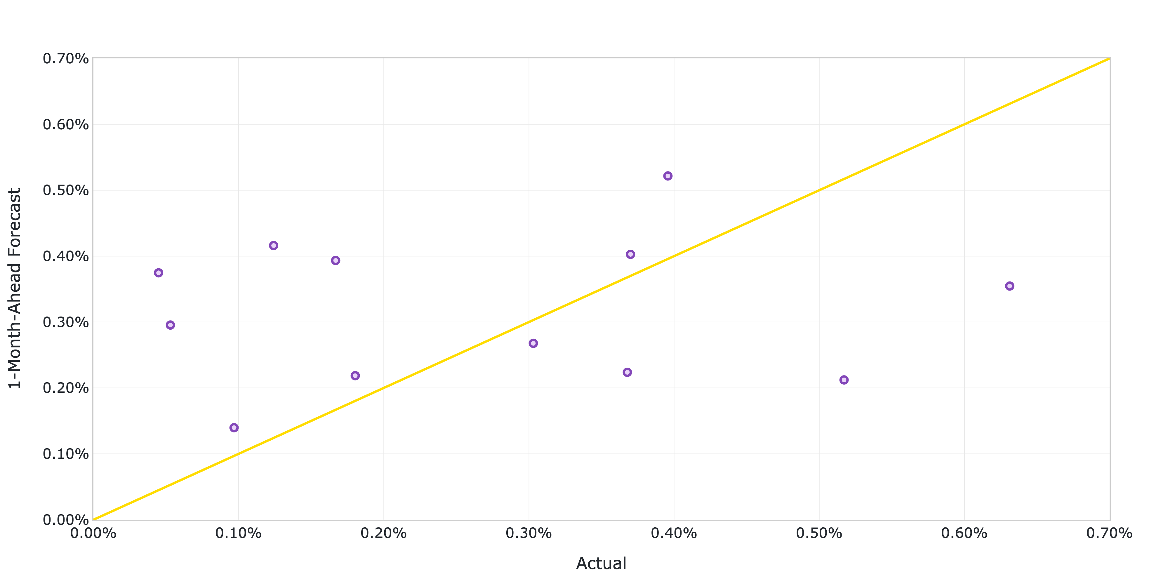
Figure 2: Actual versus predicted US CPI MoM inflation from January 2023 to December 2023.

2.5 Generate the AutoML predictions

We now run a batch transform job with the selected pipeline to generate the forecasts over the test set.

# Create the model
model = automl.create_model(
    name="us-cpi-model",
    sagemaker_session=session,
)

# Create the transformer
transformer = model.transformer(
    instance_count=1,
    instance_type="ml.m5.xlarge",
)

# Run the transform job
transformer.transform(
    data=test_data_s3_uri,
    content_type="text/csv",
)

2.6 Evaluate the AutoML prediction

After the batch transform job has completed, we can load the forecasts from S3.

# Get the AutoML predictions from S3
predictions = session.read_s3_file(
    bucket=bucket,
    key_prefix=f"{transformer.latest_transform_job.name}/test.csv.out"
)

# Cast the predictions to data frame
predictions = pd.read_csv(io.StringIO(predictions), header=None)
predictions.index = test_data.index
predictions.columns = ["Forecast"]

# Add the actual values to the data frame
predictions.insert(0, "Actual", test_data[target_name])

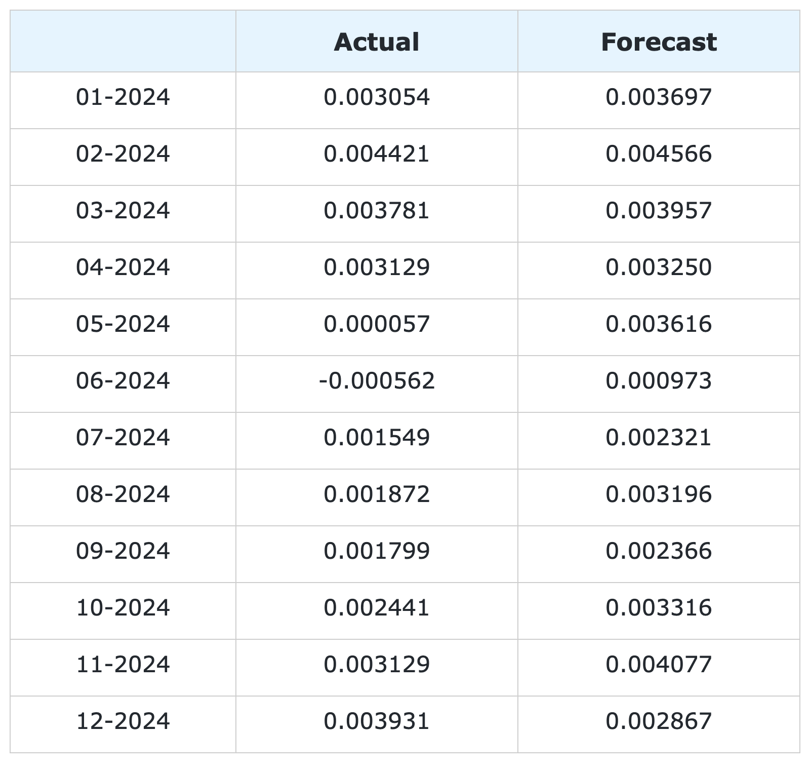
Figure 3: 1-month-ahead AutoML forecasts of US CPI MoM inflation and historical FRED-MD data.

# Calculate the error metrics
errors = pd.DataFrame({
    "RMSE": [format(root_mean_squared_error(y_true=predictions["Actual"], y_pred=predictions["Forecast"]), ".4%")],
    "MAE": [format(mean_absolute_error(y_true=predictions["Actual"], y_pred=predictions["Forecast"]), ".4%")]
})

# Calculate the correlations between the predictions and the actual values
correlations = predictions.corr()

The RMSE is 0.1322% while the MAE is 0.0978%. The forecasts display a relatively high correlation with the data (78% R-squared), even though some significant deviations are observed on a few months.

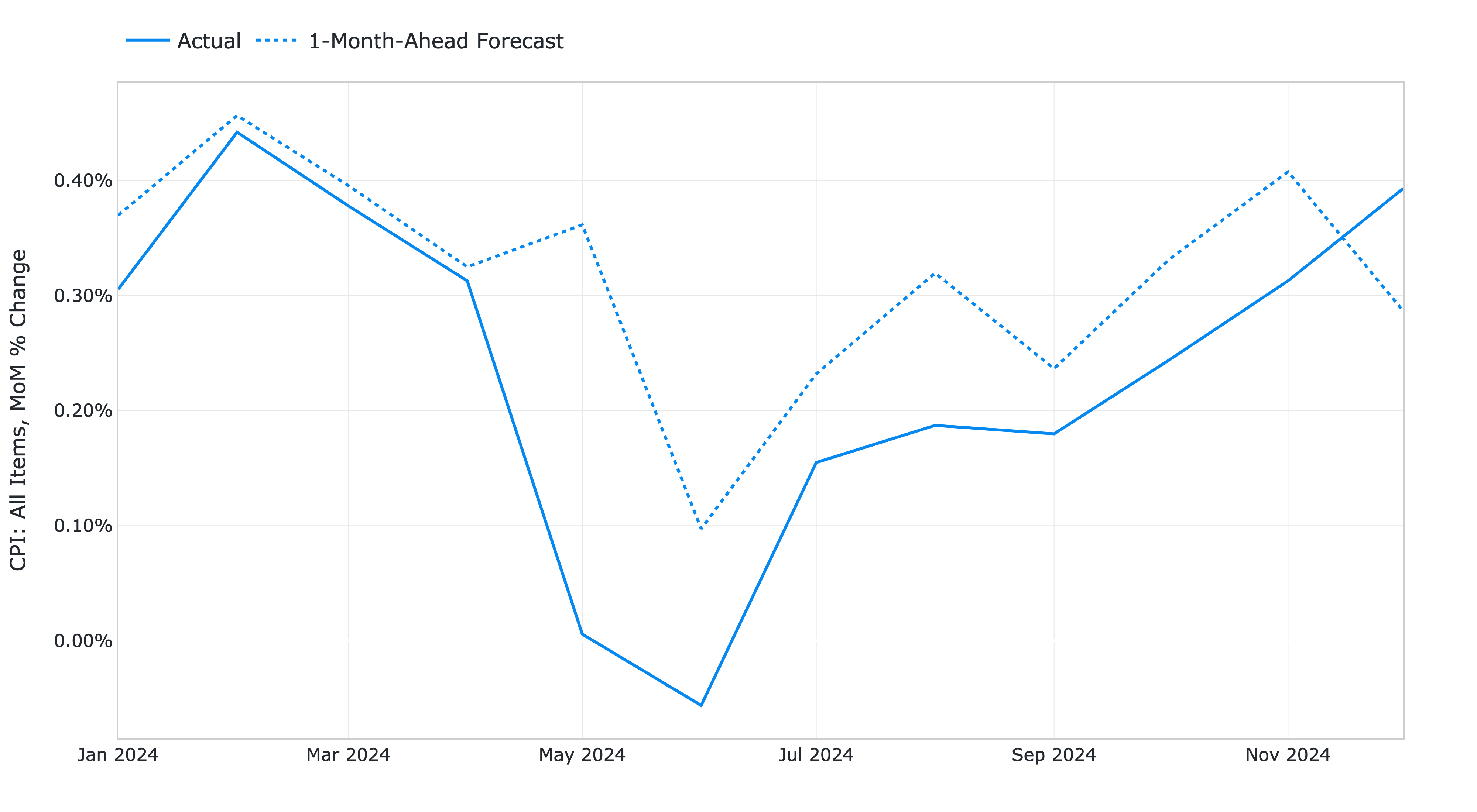
Figure 4: 1-month-ahead AutoML forecasts of US CPI MoM inflation against historical FRED-MD data from January 2024 to December 2024.

You can download the Amazon SageMaker notebook with the full code from our GitHub repository.

References

[1] Das, P., Ivkin, N., Bansal, T., Rouesnel, L., Gautier, P., Karnin, Z., Dirac, L., Ramakrishnan, L., Perunicic, A., Shcherbatyi, I. and Wu, W., (2020). Amazon SageMaker Autopilot: a white box AutoML solution at scale. In Proceedings of the Fourth International Workshop on Data Management for End-to-End Machine Learning, 1-7. doi: 10.1145/3399579.3399870.

[2] McCracken, M. W., & Ng, S. (2016). FRED-MD: A monthly database for macroeconomic research. Journal of Business & Economic Statistics, 34(4), 574-589. doi: 10.1080/07350015.2015.1086655.

[3] Medeiros, M. C., Vasconcelos, G. F., Veiga, Á., & Zilberman, E. (2021). Forecasting inflation in a data-rich environment: the benefits of machine learning methods. Journal of Business & Economic Statistics, 39(1), 98-119. doi: 10.1080/07350015.2019.1637745.

[4] Hauzenberger, N., Huber, F., & Klieber, K. (2023). Real-time inflation forecasting using non-linear dimension reduction techniques. International Journal of Forecasting, 39(2), 901-921. doi: 10.1016/j.ijforecast.2022.03.002.

[5] Paranhos, L. (2025). Predicting Inflation with Recurrent Neural Networks. International Journal of Forecasting, In press. doi: 10.1016/j.ijforecast.2024.07.010.

Appendix

Group 1: Output and Income.

Name	Description
CUMFNS	Capacity Utilization: Manufacturing
INDPRO	IP: Index
IPBUSEQ	IP: Business Equipment
IPCONGD	IP: Consumer Goods
IPDCONGD	IP: Durable Consumer Goods
IPDMAT	IP: Durable Materials
IPFINAL	IP: Final Products (Market Group)
IPFPNSS	IP: Final Products and Nonindustrial Supplies
IPFUELS	IP: Fuels
IPMANSICS	IP: Manufacturing (SIC)
IPMAT	IP: Materials
IPNCONGD	IP: Nondurable Consumer Goods
IPNMAT	IP: Nondurable Materials
IPB51222S	IP: Residential Utilities
RPI	Real Personal Income
W875RX1	Real personal Income ex Transfer Receipts

Group 2: Labor Market.

Name	Description
USCONS	All Employees: Construction
DMANEMP	All Employees: Durable goods
USFIRE	All Employees: Financial Activities
USGOOD	All Employees: Goods-Producing Industries
USGOVT	All Employees: Government
MANEMP	All Employees: Manufacturing
CES1021000001	All Employees: Mining and Logging: Mining
NDMANEMP	All Employees: Nondurable goods
USTRADE	All Employees: Retail Trade
SRVPRD	All Employees: Service-Providing Industries
PAYEMS	All Employees: Total nonfarm
USTPU	All Employees: Trade, Transportation & Utilities
USWTRADE	All Employees: Wholesale Trade
UEMPMEAN	Average Duration of Unemployment (Weeks)
CES2000000008	Average Hourly Earnings: Construction
CES0600000008	Average Hourly Earnings: Goods-Producing
CES3000000008	Average Hourly Earnings: Manufacturing
CES0600000007	Average Weekly Hours: Goods-Producing
AWHMAN	Average Weekly Hours: Manufacturing
AWOTMAN	Average Weekly Overtime Hours: Manufacturing
CE16OV	Civilian Employment
CLF16OV	Civilian Labor Force
UNRATE	Civilian Unemployment Rate
UEMP15OV	Civilians Unemployed - 15 Weeks & Over
UEMPLT5	Civilians Unemployed - Less Than 5 Weeks
UEMP15T26	Civilians Unemployed for 15-26 Weeks
UEMP27OV	Civilians Unemployed for 27 Weeks and Over
UEMP5TO14	Civilians Unemployed for 5-14 Weeks
HWI	Help-Wanted Index for United States
CLAIMSX	Initial Claims
HWIURATIO	Ratio of Help Wanted/No. Unemployed

Group 3: Consumption and Orders.

Name	Description
HOUSTMW	Housing Starts, Midwest
HOUSTNE	Housing Starts, Northeast
HOUSTS	Housing Starts, South
HOUSTW	Housing Starts, West
HOUST	Housing Starts: Total New Privately Owned
PERMIT	New Private Housing Permits (SAAR)
PERMITMW	New Private Housing Permits, Midwest (SAAR)
PERMITNE	New Private Housing Permits, Northeast (SAAR)
PERMITS	New Private Housing Permits, South (SAAR)
PERMITW	New Private Housing Permits, West (SAAR)

Group 4: Orders and Inventories.

Name	Description
UMCSENTX	Consumer Sentiment Index
ACOGNO	New Orders for Consumer Goods
AMDMNOX	New Orders for Durable Goods
ANDENOX	New Orders for Nondefense Capital Goods
CMRMTSPLX	Real Manufacturing and Trade Industries Sales
DPCERA3M086SBEA	Real Personal Consumption Expenditures
RETAILX	Retail and Food Services Sales
BUSINVX	Total Business Inventories
ISRATIOX	Total Business: Inventories to Sales Ratio
AMDMUOX	Unfilled Orders for Durable Goods

Group 5: Money and Credit

Name	Description
BUSLOANS	Commercial and Industrial Loans
DTCOLNVHFNM	Consumer Motor Vehicle Loans Outstanding
M1SL	M1 Money Stock
M2SL	M2 Money Stock
BOGMBASE	Monetary Base
CONSPI	Nonrevolving Consumer Credit to Personal Income
REALLN	Real Estate Loans at All Commercial Banks
M2REAL	Real M2 Money Stock
NONBORRES	Reserves Of Depository Institutions
INVEST	Securities in Bank Credit at All Commercial Banks
DTCTHFNM	Total Consumer Loans and Leases Outstanding
NONREVSL	Total Nonrevolving Credit
TOTRESNS	Total Reserves of Depository Institutions

Group 6: Interest Rates and Exchange Rates

Name	Description
T1YFFM	1-Year Treasury C Minus FEDFUNDS
GS1	1-Year Treasury Rate
T10YFFM	10-Year Treasury C Minus FEDFUNDS
GS10	10-Year Treasury Rate
CP3MX	3-Month AA Financial Commercial Paper Rate
COMPAPFFX	3-Month Commercial Paper Minus FEDFUNDS
TB3MS	3-Month Treasury Bill
TB3SMFFM	3-Month Treasury C Minus FEDFUNDS
T5YFFM	5-Year Treasury C Minus FEDFUNDS
GS5	5-Year Treasury Rate
TB6MS	6-Month Treasury Bill
TB6SMFFM	6-Month Treasury C Minus FEDFUNDS
EXCAUSX	Canada / U.S. Foreign Exchange Rate
FEDFUNDS	Effective Federal Funds Rate
EXJPUSX	Japan / U.S. Foreign Exchange Rate
BAAFFM	Moody’s Baa Corporate Bond Minus FEDFUNDS
AAAFFM	Moody’s Aaa Corporate Bond Minus FEDFUNDS
AAA	Moody’s Seasoned Aaa Corporate Bond Yield
BAA	Moody’s Seasoned Baa Corporate Bond Yield
EXSZUSX	Switzerland / U.S. Foreign Exchange Rate
TWEXAFEGSMTHX	Trade Weighted U.S. Dollar Index
EXUSUKX	U.S. / U.K. Foreign Exchange Rate

Group 7: Prices

Name	Description
CPIAUCSL	CPI: All Items
CPIULFSL	CPI: All Items less food
CUSR0000SA0L5	CPI: All items less medical care
CUSR0000SA0L2	CPI: All items less shelter
CPIAPPSL	CPI: Apparel
CUSR0000SAC	CPI: Commodities
CUSR0000SAD	CPI: Durables
CPIMEDSL	CPI: Medical Care
CUSR0000SAS	CPI: Services
CPITRNSL	CPI: Transportation
OILPRICEX	Crude Oil, Spliced WTI and Cushing
WPSID62	PPI: Crude Materials
WPSFD49502	PPI: Finished Consumer Goods
WPSFD49207	PPI: Finished Goods
WPSID61	PPI: Intermediate Materials
PPICMM	PPI: Metals and metal products
DDURRG3M086SBEA	Personal Consumption Expenditures: Durable goods
DNDGRG3M086SBEA	Personal Consumption Expenditures: Nondurable goods
DSERRG3M086SBEA	Personal Consumption Expenditures: Services
PCEPI	Personal Consumption Expenditures: Chain Index

Group 8: Stock Market

Name	Description
S&P 500	S&Ps Common Stock Price Index: Composite
S&P: INDUST	S&Ps Common Stock Price Index: Industrials
S&P DIV YIELD	S&Ps Composite Common Stock: Dividend Yield
S&P PE RATIO	S&Ps Composite Common Stock: Price-Earnings Ratio
VIXCLSX	VIX